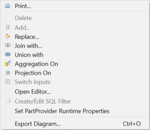
I lately looked deeper into the modeling of Composite Provider in BW/4HANA 2.0 and found some difference between a BW/4HANA 1.0, BWonHANA 7.50 and the latest version BW/4HANA 2.0. So let's compare them and see what's new, and we can go deeper in further posts. We start with the context menu of the scenario for the provider.

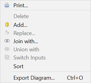
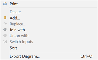
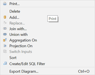
As you can see the BW/4HANA 1.0 and BWonHANA 7.5 is quite the same but BW/4HANA 2.0 has some more entries in the context menu. We now see there an Aggregation, Projection and a Create/Edit SQL Filter. Also, the join types are enhanced with Full Outer-, Referential-, Right Outer Join instead of only Inner and Left Outer Join on BW/4HANA 1.0.

You have now also some different join operations like:

• Equal to
• Greater Than or Equal to
• Greater Than
• Less Than or Equal to
• Less Than
• Not Equal to

So you can build more flexible joins.

So we have here some similar functions to a SAP HANA Calculation View? Or what can we do with it? I will build a Composite Provider with Aggregation or Projection and a SQL Filter in a demo. Now lets dive into the context menu of the mapping.

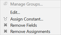
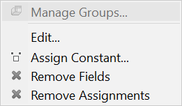
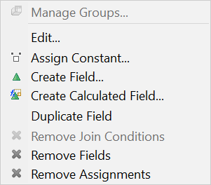
As you can see the context menu here also expanded with some new features. Like Create Field, Create Calculated Field and Duplicate Field. So what are these new things?

To say it in SAP language the two new types of nodes (Aggregation and Projection) is to simplify modeling in SAP BW/4HANA. But what can we do with it? With the Aggregation Node we can aggregate key figure values in the target structure of the Composite Provider. This is similar to the functionality which is already provided in the SAP HANA Calculation View. But we have in the Composite Provider less aggregation types than in a SAP HANA Calculation View.

The Projection Node is mainly there to define the output structure and add a filter on a specific part provider. 

We start with the function SQL Filter and see how it works. If you want to add a SQL Filter, you need either an Aggregation or a Projection on top of your part provider. Now we are able to add a SQL Filter with the HANA SQL Script language. You find the HANA SQL Script reference here.

As you can see on a part provider the function is disabled.

With Calculated Fields it is possible to enrich or refine data from part providers with additional business logic in SAP HANA SQL syntax. You can also add simple Fields as well. Both fields can be defined either as Characteristics or as a Key Figure. As a characteristic the option "Forced Group by" can also be enabled.

So let's build some different cases and see what is happening. We have 3 ADSOs with the following structure:

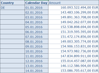
• ADSO 1: Sales DE
• • 0Country, 0CALMONTH2, 0CALYEAR, 0AMOUNT
• ADSO 2: Sales US/DE
• • 0COUNTRY, 0CALDAY, 0AMOUNT
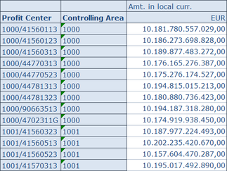
• ADSO 3: Sales Profit Center
• • 0PROFIT_CTR, 0CO_AREA, 0CALYEAR, 0CALMONTH2, 0AMONT_LC

As you can see every ADSO has a different structure and ADSO 2 has a detailed view of the data of ADSO 1. So let's look into the data:

Now we want to combine the data of ADSO 1: Sales DE with information of ADSO 2: Sales US/D as well as enhance ADSO 1 data with ADSO 3: Sales Profit Center values. So let's get started: 

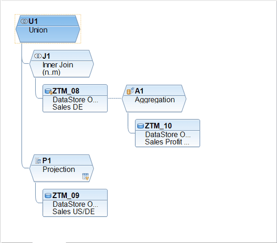
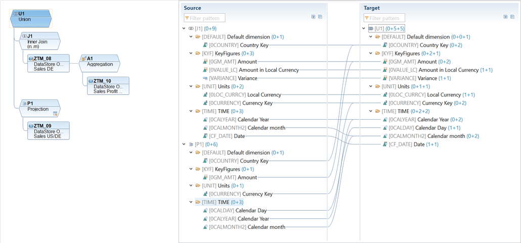
Step 1: Since our Sales DE and the Sales Profit Center have different granularity, an additional aggregation is build on top of the ADSO 3. We want to remove the Controlling Area and Profit Center information and join it with ADSO 1: Sales DE.

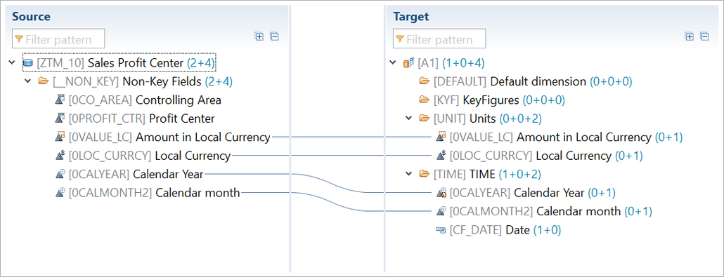
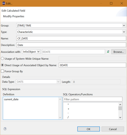
Step 2: In this example we get the current date as a calculation field as a characteristic, and we enable "Forced Group By" for 0CALYEAR.

Step 3: ADSO 1 is joined with the aggregation of our ADSO 3. Here we define a calculation field and calculate the variance between the Amount and the Amount in Local Currency. The join condition is based on 0CALYEAR and 0CALMONTH2.

Step 4: Our Sales US/DE includes the Sales from US and from DE. To avoid duplicate data with ADSO 1: Sales DE, we create a projection on top of the ADSO 2 and use SQL Filter to select only the US data. We also activate the navigation attributes 0CALMONTH2 and 0CALYEAR from 0DATE.

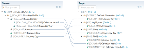
Step 5: In the UNION, we map the date field from ADSO 2: Sales US/DE to the current date from the Join. The fields 0CALMONTH2 and 0CALYEAR are mapped with from the navigational attributes of 0CALDAY.

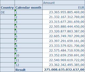
Step 6: The result is now showing in Analysis for Office. As you can see, the Sales DE ADSO is enriched to the Sales of the Profit Center ADSO. We also see the variance and the current date. The Sales from US only get the column Amount filled.

It is really cool, that we are able to build more flexible Composite Provider, but I miss a data preview function for each node. This could be a nice feature in the future. Do you like this feature? Any ideas what you can do with it?

These posts might also be interesting:

• BW/4HANA 2.0 Agile Open ODS View Modeling
• BW/4HANA 2.0 Composite Provider with InfoObject Join
• BW/4HANA 2.0 first impressions

• In my newsletter you get informed about new topics
• You learn how to use Analysis Office
• You get tips and tricks about SAP BI topics
• You get the first 3 chapters of my e-book Analysis Office - The Comprehensive Guide for free